Discrete Fourier Transform on Real Audio Data

Frequency Scaling Cosine

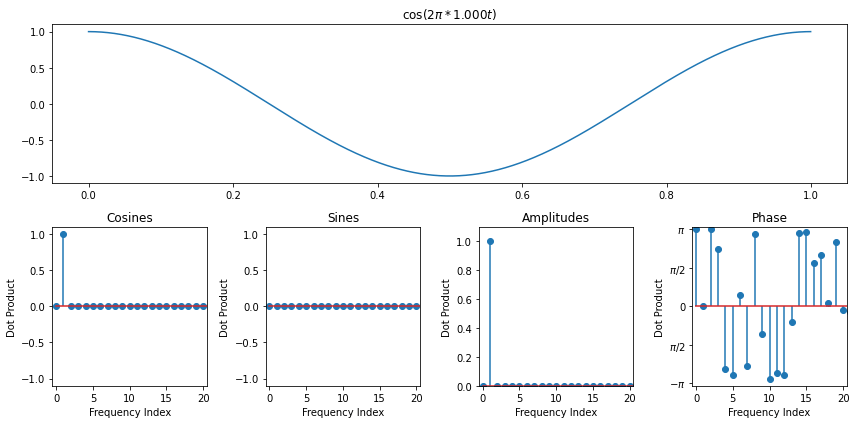
We're going to try to estimate frequencies in real signals now by using amplitudes of the discrete fourier transform. Before we do that, though, there's one caveat if the frequency that actually exists in our signal does not go through an integer number of periods over the audio that we measured. In that case, the amplitude actually splits over all frequency bins, though it's concentrated on the bins just below and just above the actualy frequency. So peak picking might still be OK

import numpy as np
import matplotlib.pyplot as plt
import librosa
import IPython.display as ipd

def get_dft(x):
    """
    Return the non-redundant real/imaginary components
    of the DFT, expressed as amplitudes of sines/cosines
    involved
    
    Parameters
    ----------
    x: ndarray(N)
        A signal
    
    Returns
    -------
    cos_sum: ndarray(ceil(N/2)), sin_sums(ndarray(ceil(N/2)))
        DFT cosine/sine amplitudes
    """
    N = len(x)
    t = np.linspace(0, 1, N+1)[0:N]
    n_freqs = int(np.ceil(N/2))
    f = np.fft.fft(x) # O(N log N) time
    cos_sums = np.real(f)[0:n_freqs]/(N/2)
    sin_sums = -np.imag(f)[0:n_freqs]/(N/2)
    return cos_sums, sin_sums

Let's write some code to compute the DFT amplitudes at each frequency index and to plot them againt their corresponding frequencies in hz. We can also estimate the note involved by finding the frequency that has a maximum amplitude and by inverting the note to frequency equation as

$n = 12 \log_2(f/440)$

Sometimes we get the note wrong by just looking at the peak, but we can at least visually see that the harmonics are spaced in a particular way. Looking for this spacing is in practice how people often visually figure out what the "fundamental frequency" is.

Below is an implementation of this technique that works well on me bowing the A string on my violin

x, sr = librosa.load("A4.wav")
c, s = get_dft(x)
amps = np.sqrt(c**2 + s**2)
ks = np.arange(len(c))
freqs = ks*sr/len(x)
idx = np.argmax(amps)
max_freq = freqs[idx]
# freq = 440*2^(note/12)
# note = log_2(freq/440)*12
note = np.round(np.log2(max_freq/440)*12) % 12
plt.plot(freqs, amps)
plt.scatter([freqs[idx]], [amps[idx]])
plt.title("Max Freq = {:.3f}, Note number = {}".format(max_freq, note))
plt.xlabel("Frequency Hz")
plt.xlim([0, 4000])
ipd.Audio(x, rate=sr)