Convolution And The DFT

Chris Tralie

import numpy as np
import matplotlib.pyplot as plt
import IPython.display as ipd
from scipy.signal import fftconvolve
import librosa

In this module, we do some experiments where we notice that the amplitude of the DFT of the convolution of two signals seems to be the product of the amplitudes of the DFTs of the original signal and the DFT of its impulse response

DFT Formulas

Forward DFT

$X[k] = \sum_{n=0}^{N-1} x[n] e^{-i 2 \pi \frac{k}{N} n}$

Inverse DFT

$x[n] = \frac{1}{N}\sum_{k=0}^{N-1} X[k] e^{i 2 \pi \frac{k}{N} n}$

Convolution Formulas

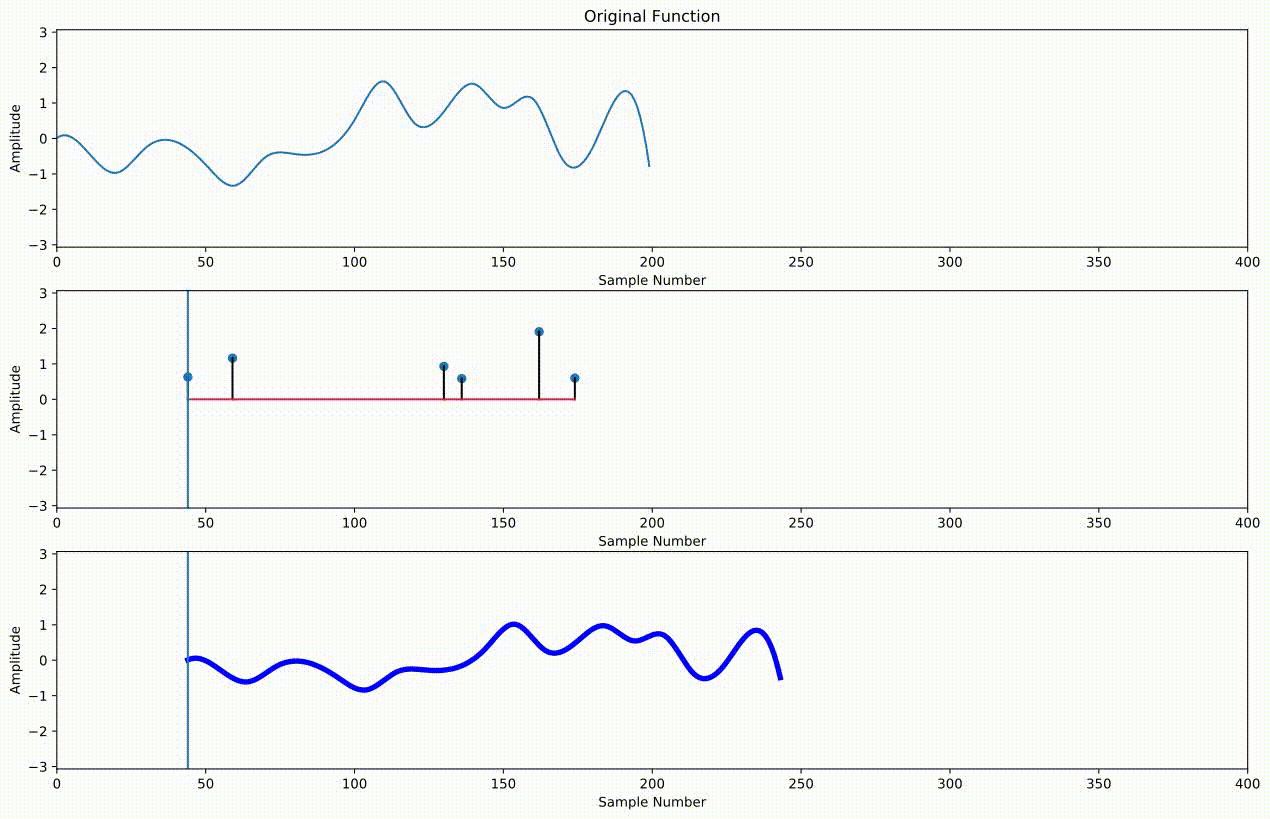
Supoose we have a signal $x[n]$ with $N$ samples, and we have an impulse response $h[j]$ with $J$ samples. Then we compute the convolution $x*h[n]$ as

$x*h[n] = \sum_{j=0}^{J-1} h[j]x[n-j] $

Convolution DFT Experiments

def plot_dft_convolution(x, h, sr):
    X = np.fft.fft(x)
    nfreqs = int(len(x)/2) # Only plot the first half of the
    # frequencies since the second half is the mirror image_on
    X = X[0:nfreqs]
    freqs = np.arange(nfreqs)*sr/len(x)


    plt.figure(figsize=(6, 8))
    plt.subplot(311)
    plt.plot(freqs, np.abs(X))
    plt.yscale('log')
    ipd.Audio(x, rate=sr)
    plt.xlim([0, 3000])
    plt.xlabel("Frequency (hz)")
    plt.title("|FFT(x)|")

    plt.subplot(312)
    H = np.fft.fft(h)
    nfreqs = int(len(h)/2) # Only plot the first half of the
    # frequencies since the second half is the mirror image_on
    H = H[0:nfreqs]
    freqs = np.arange(nfreqs)*sr/len(h)
    plt.plot(freqs, np.abs(H))
    plt.yscale("log")
    plt.xlim([0, 3000])
    plt.title("|FFT(h)|")
    plt.ylim([1e-5, 1e3])


    plt.subplot(313)
    y = fftconvolve(x, h)
    Y = np.fft.fft(y)
    nfreqs = int(len(y)/2) # Only plot the first half of the
    # frequencies since the second half is the mirror image_on
    Y = Y[0:nfreqs]
    freqs = np.arange(nfreqs)*sr/len(y)
    plt.plot(freqs, np.abs(Y))
    plt.yscale("log")
    plt.xlim([0, 3000])
    plt.title("|FFT(x*h)|")
    plt.ylim([1e-5, 1e3])
    plt.tight_layout()
    return y

x, sr = librosa.load("robot.wav", sr=44100)
ipd.Audio(x, rate=sr)

Example: Comb Filter

h = np.zeros(sr)
T = 100
h[0:5*T:T] = 1
y = plot_dft_convolution(x, h, sr)
ipd.Audio(y, rate=sr)

Example: Lowpass Filter

If we make an impulse response which is a run of 1s a the beginning, then this acts like a "lowpass filter" and muffles the higher frequencies

x = np.random.randn(sr*2)
h = np.zeros(sr)
h[0:100] = 1
h = h/np.sum(h)
plt.plot(h)
y = plot_dft_convolution(x, h, sr)
ipd.Audio(y, rate=sr)