import numpy as np
import matplotlib.pyplot as plt
import IPython.display as ipd
import librosa
import librosa.display
x, sr = librosa.load("beatles.wav")
hop_length=512
win = 4096
S = librosa.stft(x, hop_length=hop_length, n_fft=win)
S = np.abs(S)
Sdb = librosa.amplitude_to_db(S,ref=np.max)
ipd.Audio(x, rate=sr)
"Come Together," the above clip, is at 83 beats per minute (bpm)
M = Sdb.shape[0] # How many rows I have (frequency indices)
N = Sdb.shape[1] # How many columns I have (time window indices)
novfn = np.zeros(N-1) # Pre-allocate space to hold some kind of difference between columns
times = np.arange(N-1)*hop_length/sr
diff = Sdb[:, 1::] - Sdb[:, 0:-1]
diff[diff < 0] = 0 # Cut out the differences that are less than 0
novfn = np.sum(diff, axis=0)
plt.plot(times, novfn)
Autocorrelation
Given a signal $x[n]$ with $N$ samples, the autocorrelation $r[k]$ is define as
$r[k] = \sum_{n = 0}^{N-1} x[n]x[n-k]$
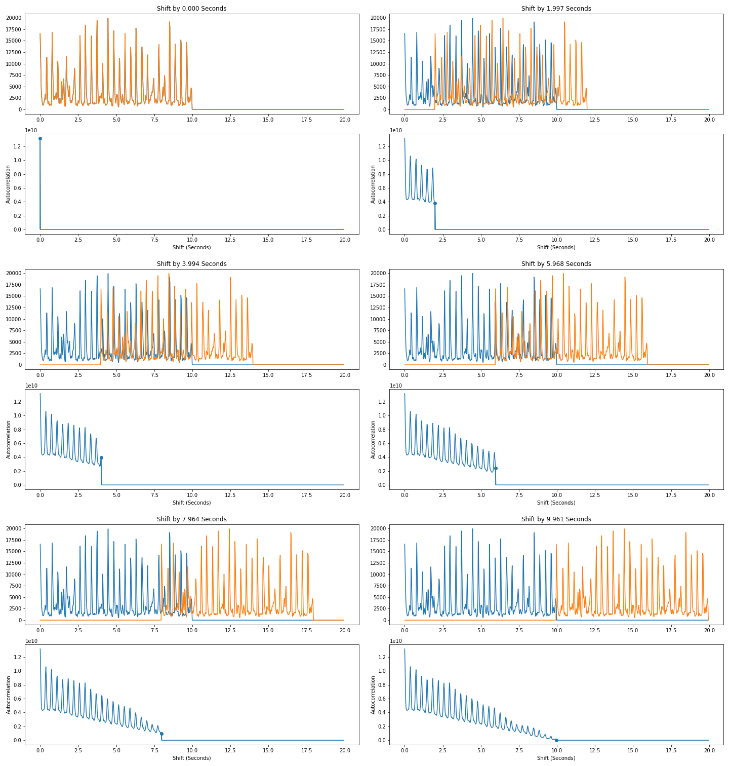
In other words, we line up a signal with itself at differents shifts and take the dot product. As shown below, when we shift by a multiple of a period, the signal lines up well with itself and the dot product is large. This leads to a periodic pattern in the autcorrelation itself

Here is a naive $O(N^2)$ algorithm to compute the autocorrelation directly from the definition
def autocorr_slow(x):
    N = len(x)
    r = np.zeros(N)
    for k in range(N):
        corr = 0
        for n in range(N):
            if n-k >= 0:
                corr += x[n]*x[n-k]
        r[k] = corr
    return r
But we can use the fact that the autocorrelation of a signal is the convolution of that signal and its reverse to compute it more quickly
def autocorr(x):
    N = len(x)
    xpad = np.zeros(N*2)
    xpad[0:N] = x
    F = np.fft.fft(xpad)
    FConv = np.real(F)**2 + np.imag(F)**2 # Fourier transform of the convolution of x and its reverse
    return np.real(np.fft.ifft(FConv)[0:N])
r = autocorr(novfn)
times = np.arange(len(r))*hop_length/sr
plt.plot(times, r)
plt.plot(times, 0.8*10**10*np.ones(len(r)))
Now let's look at the shifts of time where the autocorrelation exceeds a certain value, and convert those shifts to beats per minute. What we see is we get our 83 bpm in there, but we also get double that because of the "microbeat." We also get half of that (about 41 bpm), because if it repeats itself every beat, it repeats itself every two beats as well. And by the same reasoning, we get a quarter of it (about 20 bpm)
intervals = times[r > 0.8*10**10]
print(intervals)
bpm = 60/intervals
print(bpm)