import librosa
import numpy as np
import matplotlib.pyplot as plt
import IPython.display as ipd
In most natural audio that we record, there are a range of frequencies that occur at different times. One simple way to estimate instantaneous frequency is to count the number of zero crossings over an interval. Let's say we have the following "linear chirp" (named as such since the perceived frequency, the derivative of the inside of the cosine, increases linearly)
sr = 8000
t = np.arange(sr*2)/sr
y = np.cos(2*np.pi*220*t**2)
ipd.Audio(y, rate=sr)
If we zoom in on a small chunk of audio in the first half, we see that it crosses the x-axis 6 times
plt.plot(t[4000:4100], y[4000:4100])
plt.plot(t[4000:4100], 0*y[4000:4100])

If we zoom in later on a chunk of audio that's the same length, we see that there are 16 zero crossings, indicating that the frequency has gone up
plt.plot(t[12000:12100], y[12000:12100])
plt.plot(t[12000:12100], 0*y[12000:12100])

If we zoom in even later, we see even more zero crossings
plt.plot(t[15000:15100], y[15000:15100])
plt.plot(t[15000:15100], 0*y[15000:15100])

Computing Windowed Zero Crossings with No Loops
To compute zero crossings with no loops, we first have to understand cumulative sums. Below is an animaton showing how a cumulative sum works. It's very much like a definite integral, but for discrete data
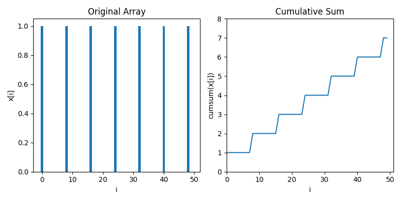
Let's move towards data that's a little bit more like zero crossings, where most of the values are zero but there's 1s spiking when stuff crosses zeros. In this case, we see the cumulative sum goes up in a staircase
Moreover, we can use the cumulative sum to count how many zero crossings there are in an interval $[a, b]$ by taking the difference of the cumulative sum at $b$ and the cumulative sum at $a$. For instance, there are 2 zero crossings between 10 and 30, which we can see as 4 - 2.
This is akin to the definite integral relationship
$\int_{a}^b f(t) dt = \int_{0}^b f(t)dt - \int_{0}^a f(t)dt $
Below is an animation showing how to compute the zeros in every possible window in a linear chirp. We see that the zero crossing counts increase linearly, so they indeed correlate with frequency
Below is the code to replicate this over a longer interval
sr = 8000
win = 200
t = np.arange(sr)/sr
y = np.cos(2*np.pi*440*t**2)

# zcs[i+1] - zcs[i]
zcs = np.sign(y)
zcs = 0.5*np.abs(zcs[1::] - zcs[0:-1])
# cusum(zcs)[i+win] - csum(zcs)[i]
zcs_win = np.cumsum(zcs)[win::] - np.cumsum(zcs)[0:-win]
plt.plot(zcs_win)

Now let's try this same thing on some real audio
y, sr = librosa.load("femalecountdown.mp3", sr=22050)
ipd.Audio(y, rate=sr)
We see that if we set all of the samples whose windows have zero crossings greater than a certain threshold, then we effectively get rid of all of the constants
y, sr = librosa.load("femalecountdown.mp3", sr=22050)
t = np.arange(len(y))/sr
win = 2000
thresh = 250

# zcs[i+1] - zcs[i]
zcs = np.sign(y)
zcs = 0.5*np.abs(zcs[1::] - zcs[0:-1])
# cusum(zcs)[i+win] - csum(zcs)[i]
zcs_win = np.cumsum(zcs)[win::] - np.cumsum(zcs)[0:-win]

y = y[int(win/2):int(win/2)+len(zcs_win)]
y[zcs_win > thresh] = 0
ipd.Audio(y, rate=sr)